Tutorials
Seràs la clau que obre tots els panys, seràs la llum, la llum il.limitada, seràs confí on l’aurora comença, seràs forment, escala il.luminada!
—Lyrics: Vicent Andrés i Estellés. Music: Ovidi Montllor, Toti Soler, M’aclame a tu
This chapter consists of a series of simple yet comprehensive tutorials that will enable you to understand PyTables’ main features. If you would like more information about some particular instance variable, global function, or method, look at the doc strings or go to the library reference in Library Reference. If you are reading this in PDF or HTML formats, follow the corresponding hyperlink near each newly introduced entity.
Please note that throughout this document the terms column and field will be used interchangeably, as will the terms row and record.
Getting started
In this section, we will see how to define our own records in Python and save collections of them (i.e. a table) into a file. Then we will select some of the data in the table using Python cuts and create NumPy arrays to store this selection as separate objects in a tree.
In examples/tutorial1-1.py you will find the working version of all the code in this section. Nonetheless, this tutorial series has been written to allow you reproduce it in a Python interactive console. I encourage you to do parallel testing and inspect the created objects (variables, docs, children objects, etc.) during the course of the tutorial!
Importing tables objects
Before starting you need to import the public objects in the tables package. You normally do that by executing:
>>> import tables
This is the recommended way to import tables if you don’t want to pollute your namespace. However, PyTables has a contained set of first-level primitives, so you may consider using the alternative:
>>> from tables import *
If you are going to work with NumPy arrays (and normally, you will) you will also need to import functions from the numpy package. So most PyTables programs begin with:
>>> import tables   # but in this tutorial we use "from tables import \*"
>>> import numpy as np
Declaring a Column Descriptor
Now, imagine that we have a particle detector and we want to create a table object in order to save data retrieved from it. You need first to define the table, the number of columns it has, what kind of object is contained in each column, and so on.
Our particle detector has a TDC (Time to Digital Converter) counter with a dynamic range of 8 bits and an ADC (Analogical to Digital Converter) with a range of 16 bits. For these values, we will define 2 fields in our record object called TDCcount and ADCcount. We also want to save the grid position in which the particle has been detected, so we will add two new fields called grid_i and grid_j. Our instrumentation also can obtain the pressure and energy of the particle. The resolution of the pressure-gauge allows us to use a single-precision float to store pressure readings, while the energy value will need a double-precision float. Finally, to track the particle we want to assign it a name to identify the kind of the particle it is and a unique numeric identifier. So we will add two more fields: name will be a string of up to 16 characters, and idnumber will be an integer of 64 bits (to allow us to store records for extremely large numbers of particles).
Having determined our columns and their types, we can now declare a new Particle class that will contain all this information:
>>> from tables import *
>>> class Particle(IsDescription):
...     name      = StringCol(16)   # 16-character String
...     idnumber  = Int64Col()      # Signed 64-bit integer
...     ADCcount  = UInt16Col()     # Unsigned short integer
...     TDCcount  = UInt8Col()      # unsigned byte
...     grid_i    = Int32Col()      # 32-bit integer
...     grid_j    = Int32Col()      # 32-bit integer
...     pressure  = Float32Col()    # float  (single-precision)
...     energy    = Float64Col()    # double (double-precision)
>>>
This definition class is self-explanatory. Basically, you declare a class variable for each field you need. As its value you assign an instance of the appropriate Col subclass, according to the kind of column defined (the data type, the length, the shape, etc). See the The Col class and its descendants for a complete description of these subclasses. See also Supported data types in PyTables for a list of data types supported by the Col constructor.
From now on, we can use Particle instances as a descriptor for our detector data table. We will see later on how to pass this object to construct the table. But first, we must create a file where all the actual data pushed into our table will be saved.
Creating a PyTables file from scratch
Use the top-level open_file() function to create a PyTables file:
>>> h5file = open_file("tutorial1.h5", mode="w", title="Test file")
open_file() is one of the objects imported by the
`from tables import *` statement. Here, we are saying that we want to
create a new file in the current working directory called “tutorial1.h5” in
“w”rite mode and with a descriptive title string (“Test file”).
This function attempts to open the file, and if successful, returns the File
(see The File Class) object instance h5file. The root of the object
tree is specified in the instance’s root attribute.
Creating a new group
Now, to better organize our data, we will create a group called detector that branches from the root node. We will save our particle data table in this group:
>>> group = h5file.create_group("/", 'detector', 'Detector information')
Here, we have taken the File instance h5file and invoked its
File.create_group() method to create a new group called detector
branching from “/” (another way to refer to the h5file.root object we
mentioned above). This will create a new Group (see The Group class)
object instance that will be assigned to the variable group.
Creating a new table
Let’s now create a Table (see The Table class) object as a branch off
the newly-created group. We do that by calling the File.create_table()
method of the h5file object:
>>> table = h5file.create_table(group, 'readout', Particle, "Readout example")
We create the Table instance under group. We assign this table the node name “readout”. The Particle class declared before is the description parameter (to define the columns of the table) and finally we set “Readout example” as the Table title. With all this information, a new Table instance is created and assigned to the variable table.
If you are curious about how the object tree looks right now, simply print the File instance variable h5file, and examine the output:
>>> print(h5file)
tutorial1.h5 (File) 'Test file'
Last modif.: 'Wed Mar  7 11:06:12 2007'
Object Tree:
/ (RootGroup) 'Test file'
/detector (Group) 'Detector information'
/detector/readout (Table(0,)) 'Readout example'
As you can see, a dump of the object tree is displayed. It’s easy to see the Group and Table objects we have just created. If you want more information, just type the variable containing the File instance:
>>> h5file
File(filename='tutorial1.h5', title='Test file', mode='w', root_uep='/', filters=Filters(complevel=0, shuffle=False, bitshuffle=False, fletcher32=False))
/ (RootGroup) 'Test file'
/detector (Group) 'Detector information'
/detector/readout (Table(0,)) 'Readout example'
description := {
  "ADCcount": UInt16Col(shape=(), dflt=0, pos=0),
  "TDCcount": UInt8Col(shape=(), dflt=0, pos=1),
  "energy": Float64Col(shape=(), dflt=0.0, pos=2),
  "grid_i": Int32Col(shape=(), dflt=0, pos=3),
  "grid_j": Int32Col(shape=(), dflt=0, pos=4),
  "idnumber": Int64Col(shape=(), dflt=0, pos=5),
  "name": StringCol(itemsize=16, shape=(), dflt='', pos=6),
  "pressure": Float32Col(shape=(), dflt=0.0, pos=7)}
  byteorder := 'little'
  chunkshape := (87,)
More detailed information is displayed about each object in the tree. Note how Particle, our table descriptor class, is printed as part of the readout table description information. In general, you can obtain much more information about the objects and their children by just printing them. That introspection capability is very useful, and I recommend that you use it extensively.
The time has come to fill this table with some values. First we will get a pointer to the Row (see The Row class) instance of this table instance:
>>> particle = table.row
The row attribute of table points to the Row instance that will be used to write data rows into the table. We write data simply by assigning the Row instance the values for each row as if it were a dictionary (although it is actually an extension class), using the column names as keys.
Below is an example of how to write rows:
>>> for i in range(10):
...     particle['name']  = f'Particle: {i:6d}'
...     particle['TDCcount'] = i % 256
...     particle['ADCcount'] = (i * 256) % (1 << 16)
...     particle['grid_i'] = i
...     particle['grid_j'] = 10 - i
...     particle['pressure'] = float(i*i)
...     particle['energy'] = float(particle['pressure'] ** 4)
...     particle['idnumber'] = i * (2 ** 34)
...     # Insert a new particle record
...     particle.append()
>>>
This code should be easy to understand. The lines inside the loop just assign values to the different columns in the Row instance particle (see The Row class). A call to its append() method writes this information to the table I/O buffer.
After we have processed all our data, we should flush the table’s I/O buffer if we want to write all this data to disk. We achieve that by calling the table.flush() method:
>>> table.flush()
Remember, flushing a table is a very important step as it will not only help to maintain the integrity of your file, but also will free valuable memory resources (i.e. internal buffers) that your program may need for other things.
Reading (and selecting) data in a table
Ok. We have our data on disk, and now we need to access it and select from specific columns the values we are interested in. See the example below:
>>> table = h5file.root.detector.readout
>>> pressure = [x['pressure'] for x in table.iterrows() if x['TDCcount'] > 3 and 20 <= x['pressure'] < 50]
>>> pressure
[25.0, 36.0, 49.0]
The first line creates a “shortcut” to the readout table deeper on the object tree. As you can see, we use the natural naming schema to access it. We also could have used the h5file.get_node() method, as we will do later on.
You will recognize the last two lines as a Python list comprehension.
It loops over the rows in table as they are provided by the
Table.iterrows() iterator. The iterator returns values until all the
data in table is exhausted. These rows are filtered using the expression:
x['TDCcount'] > 3 and 20 <= x['pressure'] < 50
So, we are selecting the values of the pressure column from filtered records to create the final list and assign it to pressure variable.
We could have used a normal for loop to accomplish the same purpose, but I find comprehension syntax to be more compact and elegant.
PyTables do offer other, more powerful ways of performing selections which
may be more suitable if you have very large tables or if you need very high
query speeds. They are called in-kernel and indexed queries, and you can
use them through Table.where() and other related methods.
Let’s use an in-kernel selection to query the name column for the same set of cuts:
>>> names = [ x['name'] for x in table.where("""(TDCcount > 3) & (20 <= pressure) & (pressure < 50)""") ]
>>> names
['Particle:      5', 'Particle:      6', 'Particle:      7']
In-kernel and indexed queries are not only much faster, but as you can see, they also look more compact, and are among the greatest features for PyTables, so be sure that you use them a lot. See Condition Syntax and Accelerating your searches for more information on in-kernel and indexed selections.
Note
A special care should be taken when the query condition includes string literals. Indeed Python 2 string literals are string of bytes while Python 3 strings are unicode objects.
With reference to the above definition of Particle it has to be
noted that the type of the “name” column do not change depending on the
Python version used (of course).
It always corresponds to strings of bytes.
Any condition involving the “name” column should be written using the
appropriate type for string literals in order to avoid
TypeErrors.
Suppose one wants to get rows corresponding to specific particle names.
The code below will work fine in Python 2 but will fail with a
TypeError in Python 3:
>>> condition = '(name == "Particle:      5") | (name == "Particle:      7")'
>>> for record in table.where(condition):  # TypeError in Python3
...     # do something with "record"
The reason is that in Python 3 “condition” implies a comparison between a string of bytes (“name” column contents) and an unicode literals.
The correct way to write the condition is:
>>> condition = '(name == b"Particle: 5") | (name == b"Particle: 7")'
That’s enough about selections for now. The next section will show you how to save these selected results to a file.
Creating new array objects
In order to separate the selected data from the mass of detector data, we will create a new group columns branching off the root group. Afterwards, under this group, we will create two arrays that will contain the selected data. First, we create the group:
>>> gcolumns = h5file.create_group(h5file.root, "columns", "Pressure and Name")
Note that this time we have specified the first parameter using natural naming (h5file.root) instead of with an absolute path string (“/”).
Now, create the first of the two Array objects we’ve just mentioned:
>>> h5file.create_array(gcolumns, 'pressure', np.array(pressure), "Pressure column selection")
/columns/pressure (Array(3,)) 'Pressure column selection'
  atom := Float64Atom(shape=(), dflt=0.0)
  maindim := 0
  flavor := 'numpy'
  byteorder := 'little'
  chunkshape := None
We already know the first two parameters of the File.create_array()
methods (these are the same as the first two in create_table): they are the
parent group where Array will be created and the Array instance name.
The third parameter is the object we want to save to disk. In this case, it
is a NumPy array that is built from the selection list we created before.
The fourth parameter is the title.
Now, we will save the second array. It contains the list of strings we selected before: we save this object as-is, with no further conversion:
>>> h5file.create_array(gcolumns, 'name', names, "Name column selection")
/columns/name (Array(3,)) 'Name column selection'
  atom := StringAtom(itemsize=16, shape=(), dflt='')
  maindim := 0
  flavor := 'python'
  byteorder := 'irrelevant'
  chunkshape := None
As you can see, File.create_array() accepts names (which is a regular
Python list) as an object parameter. Actually, it accepts a variety of
different regular objects (see create_array()) as parameters. The flavor
attribute (see the output above) saves the original kind of object that was
saved. Based on this flavor, PyTables will be able to retrieve exactly the
same object from disk later on.
Note that in these examples, the create_array method returns an Array instance that is not assigned to any variable. Don’t worry, this is intentional to show the kind of object we have created by displaying its representation. The Array objects have been attached to the object tree and saved to disk, as you can see if you print the complete object tree:
>>> print(h5file)
tutorial1.h5 (File) 'Test file'
Last modif.: 'Wed Mar  7 19:40:44 2007'
Object Tree:
/ (RootGroup) 'Test file'
/columns (Group) 'Pressure and Name'
/columns/name (Array(3,)) 'Name column selection'
/columns/pressure (Array(3,)) 'Pressure column selection'
/detector (Group) 'Detector information'
/detector/readout (Table(10,)) 'Readout example'
Closing the file and looking at its content
To finish this first tutorial, we use the close method of the h5file File object to close the file before exiting Python:
>>> h5file.close()
>>> ^D
$
You have now created your first PyTables file with a table and two arrays. You can examine it with any generic HDF5 tool, such as h5dump or h5ls. Here is what the tutorial1.h5 looks like when read with the h5ls program.
$ h5ls -rd tutorial1.h5
/columns                 Group
/columns/name            Dataset {3}
    Data:
        (0) "Particle:      5", "Particle:      6", "Particle:      7"
/columns/pressure        Dataset {3}
    Data:
        (0) 25, 36, 49
/detector                Group
/detector/readout        Dataset {10/Inf}
    Data:
        (0) {0, 0, 0, 0, 10, 0, "Particle:      0", 0},
        (1) {256, 1, 1, 1, 9, 17179869184, "Particle:      1", 1},
        (2) {512, 2, 256, 2, 8, 34359738368, "Particle:      2", 4},
        (3) {768, 3, 6561, 3, 7, 51539607552, "Particle:      3", 9},
        (4) {1024, 4, 65536, 4, 6, 68719476736, "Particle:      4", 16},
        (5) {1280, 5, 390625, 5, 5, 85899345920, "Particle:      5", 25},
        (6) {1536, 6, 1679616, 6, 4, 103079215104, "Particle:      6", 36},
        (7) {1792, 7, 5764801, 7, 3, 120259084288, "Particle:      7", 49},
        (8) {2048, 8, 16777216, 8, 2, 137438953472, "Particle:      8", 64},
        (9) {2304, 9, 43046721, 9, 1, 154618822656, "Particle:      9", 81}
Here’s the output as displayed by the “ptdump” PyTables utility (located in utils/ directory).
$ ptdump tutorial1.h5
/ (RootGroup) 'Test file'
/columns (Group) 'Pressure and Name'
/columns/name (Array(3,)) 'Name column selection'
/columns/pressure (Array(3,)) 'Pressure column selection'
/detector (Group) 'Detector information'
/detector/readout (Table(10,)) 'Readout example'
You can pass the -v or -d options to ptdump if you want more verbosity. Try them out!
Also, in Figure 1, you can admire how the tutorial1.h5 looks like using the ViTables graphical interface.
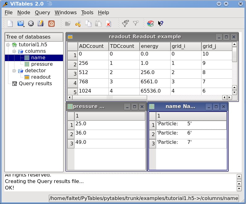
Figure 1. The initial version of the data file for tutorial 1, with a view of the data objects.
Browsing the object tree
In this section, we will learn how to browse the tree and retrieve data and also meta-information about the actual data.
In examples/tutorial1-2.py you will find the working version of all the code in this section. As before, you are encouraged to use a python shell and inspect the object tree during the course of the tutorial.
Traversing the object tree
Let’s start by opening the file we created in last tutorial section:
>>> h5file = open_file("tutorial1.h5", "a")
This time, we have opened the file in “a”ppend mode. We use this mode to add more information to the file.
PyTables, following the Python tradition, offers powerful introspection capabilities, i.e. you can easily ask information about any component of the object tree as well as search the tree.
To start with, you can get a preliminary overview of the object tree by simply printing the existing File instance:
>>> print(h5file)
tutorial1.h5 (File) 'Test file'
Last modif.: 'Wed Mar  7 19:50:57 2007'
Object Tree:
/ (RootGroup) 'Test file'
/columns (Group) 'Pressure and Name'
/columns/name (Array(3,)) 'Name column selection'
/columns/pressure (Array(3,)) 'Pressure column selection'
/detector (Group) 'Detector information'
/detector/readout (Table(10,)) 'Readout example'
It looks like all of our objects are there. Now let’s make use of the File iterator to see how to list all the nodes in the object tree:
>>> for node in h5file:
...     print(node)
/ (RootGroup) 'Test file'
/columns (Group) 'Pressure and Name'
/detector (Group) 'Detector information'
/columns/name (Array(3,)) 'Name column selection'
/columns/pressure (Array(3,)) 'Pressure column selection'
/detector/readout (Table(10,)) 'Readout example'
We can use the File.walk_groups() method of the File class to list only
the groups on tree:
>>> for group in h5file.walk_groups():
...     print(group)
/ (RootGroup) 'Test file'
/columns (Group) 'Pressure and Name'
/detector (Group) 'Detector information'
Note that File.walk_groups() actually returns an iterator, not a list
of objects. Using this iterator with the list_nodes() method is a powerful
combination. Let’s see an example listing of all the arrays in the tree:
>>> for group in h5file.walk_groups("/"):
...     for array in h5file.list_nodes(group, classname='Array'):
...         print(array)
/columns/name (Array(3,)) 'Name column selection'
/columns/pressure (Array(3,)) 'Pressure column selection'
File.list_nodes() returns a list containing all the nodes hanging off a
specific Group. If the classname keyword is specified, the method will
filter out all instances which are not descendants of the class. We have
asked for only Array instances. There exist also an iterator counterpart
called File.iter_nodes() that might be handy is some situations, like
for example when dealing with groups with a large number of nodes behind it.
We can combine both calls by using the File.walk_nodes() special method
of the File object. For example:
>>> for array in h5file.walk_nodes("/", "Array"):
...     print(array)
/columns/name (Array(3,)) 'Name column selection'
/columns/pressure (Array(3,)) 'Pressure column selection'
This is a nice shortcut when working interactively.
Finally, we will list all the Leaf, i.e. Table and Array instances (see The Leaf class for detailed information on Leaf class), in the /detector group. Note that only one instance of the Table class (i.e. readout) will be selected in this group (as should be the case):
>>> for leaf in h5file.root.detector._f_walknodes('Leaf'):
...     print(leaf)
/detector/readout (Table(10,)) 'Readout example'
We have used a call to the Group._f_walknodes() method, using the
natural naming path specification.
Of course you can do more sophisticated node selections using these powerful methods. But first, let’s take a look at some important PyTables object instance variables.
Setting and getting user attributes
PyTables provides an easy and concise way to complement the meaning of your node objects on the tree by using the AttributeSet class (see The AttributeSet class). You can access this object through the standard attribute attrs in Leaf nodes and _v_attrs in Group nodes.
For example, let’s imagine that we want to save the date indicating when the data in /detector/readout table has been acquired, as well as the temperature during the gathering process:
>>> table = h5file.root.detector.readout
>>> table.attrs.gath_date = "Wed, 06/12/2003 18:33"
>>> table.attrs.temperature = 18.4
>>> table.attrs.temp_scale = "Celsius"
Now, let’s set a somewhat more complex attribute in the /detector group:
>>> detector = h5file.root.detector
>>> detector._v_attrs.stuff = [5, (2.3, 4.5), "Integer and tuple"]
Note how the AttributeSet instance is accessed with the _v_attrs attribute because detector is a Group node. In general, you can save any standard Python data structure as an attribute node. See The AttributeSet class for a more detailed explanation of how they are serialized for export to disk.
Retrieving the attributes is equally simple:
>>> table.attrs.gath_date
'Wed, 06/12/2003 18:33'
>>> table.attrs.temperature
18.399999999999999
>>> table.attrs.temp_scale
'Celsius'
>>> detector._v_attrs.stuff
[5, (2.2999999999999998, 4.5), 'Integer and tuple']
You can probably guess how to delete attributes:
>>> del table.attrs.gath_date
If you want to examine the current user attribute set of /detector/table, you can print its representation (try hitting the TAB key twice if you are on a Unix Python console with the rlcompleter module active):
>>> table.attrs
/detector/readout._v_attrs (AttributeSet), 23 attributes:
    [CLASS := 'TABLE',
     FIELD_0_FILL := 0,
     FIELD_0_NAME := 'ADCcount',
     FIELD_1_FILL := 0,
     FIELD_1_NAME := 'TDCcount',
     FIELD_2_FILL := 0.0,
     FIELD_2_NAME := 'energy',
     FIELD_3_FILL := 0,
     FIELD_3_NAME := 'grid_i',
     FIELD_4_FILL := 0,
     FIELD_4_NAME := 'grid_j',
     FIELD_5_FILL := 0,
     FIELD_5_NAME := 'idnumber',
     FIELD_6_FILL := '',
     FIELD_6_NAME := 'name',
     FIELD_7_FILL := 0.0,
     FIELD_7_NAME := 'pressure',
     FLAVOR := 'numpy',
     NROWS := 10,
     TITLE := 'Readout example',
     VERSION := '2.6',
     temp_scale := 'Celsius',
     temperature := 18.399999999999999]
We’ve got all the attributes (including the system attributes). You can get a list of all attributes or only the user or system attributes with the _f_list() method:
>>> print(table.attrs._f_list("all"))
['CLASS', 'FIELD_0_FILL', 'FIELD_0_NAME', 'FIELD_1_FILL', 'FIELD_1_NAME',
'FIELD_2_FILL', 'FIELD_2_NAME', 'FIELD_3_FILL', 'FIELD_3_NAME', 'FIELD_4_FILL',
'FIELD_4_NAME', 'FIELD_5_FILL', 'FIELD_5_NAME', 'FIELD_6_FILL', 'FIELD_6_NAME',
'FIELD_7_FILL', 'FIELD_7_NAME', 'FLAVOR', 'NROWS', 'TITLE', 'VERSION',
'temp_scale', 'temperature']
>>> print(table.attrs._f_list("user"))
['temp_scale', 'temperature']
>>> print(table.attrs._f_list("sys"))
['CLASS', 'FIELD_0_FILL', 'FIELD_0_NAME', 'FIELD_1_FILL', 'FIELD_1_NAME',
'FIELD_2_FILL', 'FIELD_2_NAME', 'FIELD_3_FILL', 'FIELD_3_NAME', 'FIELD_4_FILL',
'FIELD_4_NAME', 'FIELD_5_FILL', 'FIELD_5_NAME', 'FIELD_6_FILL', 'FIELD_6_NAME',
'FIELD_7_FILL', 'FIELD_7_NAME', 'FLAVOR', 'NROWS', 'TITLE', 'VERSION']
You can also rename attributes:
>>> table.attrs._f_rename("temp_scale","tempScale")
>>> print(table.attrs._f_list())
['tempScale', 'temperature']
And, from PyTables 2.0 on, you are allowed also to set, delete or rename system attributes:
>>> table.attrs._f_rename("VERSION", "version")
>>> table.attrs.VERSION
Traceback (most recent call last):
    File "<stdin>", line 1, in <module>
    File "tables/attributeset.py", line 222, in __getattr__
        (name, self._v__nodepath)
AttributeError: Attribute 'VERSION' does not exist in node: '/detector/readout'
>>> table.attrs.version
'2.6'
Caveat emptor: you must be careful when modifying system attributes because you may end fooling PyTables and ultimately getting unwanted behaviour. Use this only if you know what are you doing.
So, given the caveat above, we will proceed to restore the original name of VERSION attribute:
>>> table.attrs._f_rename("version", "VERSION")
>>> table.attrs.VERSION
'2.6'
Ok, that’s better. If you would terminate your session now, you would be able to use the h5ls command to read the /detector/readout attributes from the file written to disk.
$ h5ls -vr tutorial1.h5/detector/readout
Opened "tutorial1.h5" with sec2 driver.
/detector/readout        Dataset {10/Inf}
    Attribute: CLASS     scalar
        Type:      6-byte null-terminated ASCII string
        Data:  "TABLE"
    Attribute: VERSION   scalar
        Type:      4-byte null-terminated ASCII string
        Data:  "2.6"
    Attribute: TITLE     scalar
        Type:      16-byte null-terminated ASCII string
        Data:  "Readout example"
    Attribute: NROWS     scalar
        Type:      native long long
        Data:  10
    Attribute: FIELD_0_NAME scalar
        Type:      9-byte null-terminated ASCII string
        Data:  "ADCcount"
    Attribute: FIELD_1_NAME scalar
        Type:      9-byte null-terminated ASCII string
        Data:  "TDCcount"
    Attribute: FIELD_2_NAME scalar
        Type:      7-byte null-terminated ASCII string
        Data:  "energy"
    Attribute: FIELD_3_NAME scalar
        Type:      7-byte null-terminated ASCII string
        Data:  "grid_i"
    Attribute: FIELD_4_NAME scalar
        Type:      7-byte null-terminated ASCII string
        Data:  "grid_j"
    Attribute: FIELD_5_NAME scalar
        Type:      9-byte null-terminated ASCII string
        Data:  "idnumber"
    Attribute: FIELD_6_NAME scalar
        Type:      5-byte null-terminated ASCII string
        Data:  "name"
    Attribute: FIELD_7_NAME scalar
        Type:      9-byte null-terminated ASCII string
        Data:  "pressure"
    Attribute: FLAVOR    scalar
        Type:      5-byte null-terminated ASCII string
        Data:  "numpy"
    Attribute: tempScale scalar
        Type:      7-byte null-terminated ASCII string
        Data:  "Celsius"
    Attribute: temperature scalar
        Type:      native double
        Data:  18.4
    Location:  0:1:0:1952
    Links:     1
    Modified:  2006-12-11 10:35:13 CET
    Chunks:    {85} 3995 bytes
    Storage:   470 logical bytes, 3995 allocated bytes, 11.76% utilization
    Type:      struct {
                    "ADCcount"         +0    native unsigned short
                    "TDCcount"         +2    native unsigned char
                    "energy"           +3    native double
                    "grid_i"           +11   native int
                    "grid_j"           +15   native int
                    "idnumber"         +19   native long long
                    "name"             +27   16-byte null-terminated ASCII string
                    "pressure"         +43   native float
                } 47 bytes
Attributes are a useful mechanism to add persistent (meta) information to your data.
Starting with PyTables 3.9.0, you can also set, delete, or rename attributes on individual columns. The API is designed to behave the same way as attributes on a table:
>>> table.cols.pressure.attrs['units'] = 'kPa'
>>> table.cols.energy.attrs['units'] = 'MeV'
Getting object metadata
Each object in PyTables has metadata information about the data in the file. Normally this meta-information is accessible through the node instance variables. Let’s take a look at some examples:
>>> print("Object:", table)
Object: /detector/readout (Table(10,)) 'Readout example'
>>> print("Table name:", table.name)
Table name: readout
>>> print("Table title:", table.title)
Table title: Readout example
>>> print("Number of rows in table:", table.nrows)
Number of rows in table: 10
>>> print("Table variable names with their type and shape:")
Table variable names with their type and shape:
>>> for name in table.colnames:
...     print(name, ':= %s, %s' % (table.coldtypes[name], table.coldtypes[name].shape))
ADCcount := uint16, ()
TDCcount := uint8, ()
energy := float64, ()
grid_i := int32, ()
grid_j := int32, ()
idnumber := int64, ()
name := |S16, ()
pressure := float32, ()
Here, the name, title, nrows, colnames and coldtypes attributes (see
Table for a complete attribute list) of the Table object gives us
quite a bit of information about the table data.
You can interactively retrieve general information about the public objects in PyTables by asking for help:
>>> help(table)
Help on Table in module tables.table:
class Table(tableextension.Table, tables.leaf.Leaf)
|  This class represents heterogeneous datasets in an HDF5 file.
|
|  Tables are leaves (see the `Leaf` class) whose data consists of a
|  unidimensional sequence of *rows*, where each row contains one or
|  more *fields*.  Fields have an associated unique *name* and
|  *position*, with the first field having position 0.  All rows have
|  the same fields, which are arranged in *columns*.
[snip]
|
|  Instance variables
|  ------------------
|
|  The following instance variables are provided in addition to those
|  in `Leaf`.  Please note that there are several `col` dictionaries
|  to ease retrieving information about a column directly by its path
|  name, avoiding the need to walk through `Table.description` or
|  `Table.cols`.
|
|  autoindex
|      Automatically keep column indexes up to date?
|
|      Setting this value states whether existing indexes should be
|      automatically updated after an append operation or recomputed
|      after an index-invalidating operation (i.e. removal and
|      modification of rows).  The default is true.
[snip]
|  rowsize
|      The size in bytes of each row in the table.
|
|  Public methods -- reading
|  -------------------------
|
|  * col(name)
|  * iterrows([start][, stop][, step])
|  * itersequence(sequence)
* itersorted(sortby[, checkCSI][, start][, stop][, step])
|  * read([start][, stop][, step][, field][, coords])
|  * read_coordinates(coords[, field])
* read_sorted(sortby[, checkCSI][, field,][, start][, stop][, step])
|  * __getitem__(key)
|  * __iter__()
|
|  Public methods -- writing
|  -------------------------
|
|  * append(rows)
|  * modify_column([start][, stop][, step][, column][, colname])
[snip]
Try getting help with other object docs by yourself:
>>> help(h5file)
>>> help(table.remove_rows)
To examine metadata in the /columns/pressure Array object:
>>> pressureObject = h5file.get_node("/columns", "pressure")
>>> print("Info on the object:", repr(pressureObject))
Info on the object: /columns/pressure (Array(3,)) 'Pressure column selection'
  atom := Float64Atom(shape=(), dflt=0.0)
  maindim := 0
  flavor := 'numpy'
  byteorder := 'little'
  chunkshape := None
>>> print("  shape: ==>", pressureObject.shape)
  shape: ==> (3,)
>>> print("  title: ==>", pressureObject.title)
  title: ==> Pressure column selection
>>> print("  atom: ==>", pressureObject.atom)
  atom: ==> Float64Atom(shape=(), dflt=0.0)
Observe that we have used the File.get_node() method of the File class
to access a node in the tree, instead of the natural naming method. Both are
useful, and depending on the context you will prefer one or the other.
File.get_node() has the advantage that it can get a node from the
pathname string (as in this example) and can also act as a filter to show
only nodes in a particular location that are instances of class classname.
In general, however, I consider natural naming to be more elegant and easier
to use, especially if you are using the name completion capability present in
interactive console. Try this powerful combination of natural naming and
completion capabilities present in most Python consoles, and see how pleasant
it is to browse the object tree (well, as pleasant as such an activity can
be).
If you look at the type attribute of the pressureObject object, you can
verify that it is a “float64” array. By looking at its shape attribute, you
can deduce that the array on disk is unidimensional and has 3 elements.
See Array or the internal doc strings for the complete Array
attribute list.
Reading data from Array objects
Once you have found the desired Array, use the read() method of the Array object to retrieve its data:
>>> pressureArray = pressureObject.read()
>>> pressureArray
array([ 25.,  36.,  49.])
>>> print("pressureArray is an object of type:", type(pressureArray))
pressureArray is an object of type: <type 'numpy.ndarray'>
>>> nameArray = h5file.root.columns.name.read()
>>> print("nameArray is an object of type:", type(nameArray))
nameArray is an object of type: <type 'list'>
>>>
>>> print("Data on arrays nameArray and pressureArray:")
Data on arrays nameArray and pressureArray:
>>> for i in range(pressureObject.shape[0]):
...     print(nameArray[i], "-->", pressureArray[i])
Particle:      5 --> 25.0
Particle:      6 --> 36.0
Particle:      7 --> 49.0
You can see that the Array.read() method returns an authentic NumPy
object for the pressureObject instance by looking at the output of the type()
call. A read() of the nameArray object instance returns a native Python list
(of strings). The type of the object saved is stored as an HDF5 attribute
(named FLAVOR) for objects on disk. This attribute is then read as Array
meta-information (accessible through in the Array.attrs.FLAVOR variable),
enabling the read array to be converted into the original object. This
provides a means to save a large variety of objects as arrays with the
guarantee that you will be able to later recover them in their original form.
See File.create_array() for a complete list of supported objects for the
Array object class.
Commiting data to tables and arrays
We have seen how to create tables and arrays and how to browse both data and metadata in the object tree. Let’s examine more closely now one of the most powerful capabilities of PyTables, namely, how to modify already created tables and arrays [1]
Appending data to an existing table
Now, let’s have a look at how we can add records to an existing table on disk. Let’s use our well-known readout Table object and append some new values to it:
>>> table = h5file.root.detector.readout
>>> particle = table.row
>>> for i in range(10, 15):
...     particle['name']  = f'Particle: {i:6d}'
...     particle['TDCcount'] = i % 256
...     particle['ADCcount'] = (i * 256) % (1 << 16)
...     particle['grid_i'] = i
...     particle['grid_j'] = 10 - i
...     particle['pressure'] = float(i*i)
...     particle['energy'] = float(particle['pressure'] ** 4)
...     particle['idnumber'] = i * (2 ** 34)
...     particle.append()
>>> table.flush()
It’s the same method we used to fill a new table. PyTables knows that this table is on disk, and when you add new records, they are appended to the end of the table [2].
If you look carefully at the code you will see that we have used the table.row attribute to create a table row and fill it with the new values. Each time that its append() method is called, the actual row is committed to the output buffer and the row pointer is incremented to point to the next table record. When the buffer is full, the data is saved on disk, and the buffer is reused again for the next cycle.
Caveat emptor: Do not forget to always call the flush() method after a write operation, or else your tables will not be updated!
Let’s have a look at some rows in the modified table and verify that our new data has been appended:
>>> for r in table.iterrows():
...     print("%-16s | %11.1f | %11.4g | %6d | %6d | %8d \|" % \\
...         (r['name'], r['pressure'], r['energy'], r['grid_i'], r['grid_j'],
...         r['TDCcount']))
Particle:      0 |         0.0 |           0 |      0 |     10 |        0 |
Particle:      1 |         1.0 |           1 |      1 |      9 |        1 |
Particle:      2 |         4.0 |         256 |      2 |      8 |        2 |
Particle:      3 |         9.0 |        6561 |      3 |      7 |        3 |
Particle:      4 |        16.0 |   6.554e+04 |      4 |      6 |        4 |
Particle:      5 |        25.0 |   3.906e+05 |      5 |      5 |        5 |
Particle:      6 |        36.0 |    1.68e+06 |      6 |      4 |        6 |
Particle:      7 |        49.0 |   5.765e+06 |      7 |      3 |        7 |
Particle:      8 |        64.0 |   1.678e+07 |      8 |      2 |        8 |
Particle:      9 |        81.0 |   4.305e+07 |      9 |      1 |        9 |
Particle:     10 |       100.0 |       1e+08 |     10 |      0 |       10 |
Particle:     11 |       121.0 |   2.144e+08 |     11 |     -1 |       11 |
Particle:     12 |       144.0 |     4.3e+08 |     12 |     -2 |       12 |
Particle:     13 |       169.0 |   8.157e+08 |     13 |     -3 |       13 |
Particle:     14 |       196.0 |   1.476e+09 |     14 |     -4 |       14 |
Modifying data in tables
Ok, until now, we’ve been only reading and writing (appending) values to our tables. But there are times that you need to modify your data once you have saved it on disk (this is specially true when you need to modify the real world data to adapt your goals ;). Let’s see how we can modify the values that were saved in our existing tables. We will start modifying single cells in the first row of the Particle table:
>>> print("Before modif-->", table[0])
Before modif--> (0, 0, 0.0, 0, 10, 0L, 'Particle:      0', 0.0)
>>> table.cols.TDCcount[0] = 1
>>> print("After modifying first row of ADCcount-->", table[0])
After modifying first row of ADCcount--> (0, 1, 0.0, 0, 10, 0L, 'Particle:      0', 0.0)
>>> table.cols.energy[0] = 2
>>> print("After modifying first row of energy-->", table[0])
After modifying first row of energy--> (0, 1, 2.0, 0, 10, 0L, 'Particle:      0', 0.0)
We can modify complete ranges of columns as well:
>>> table.cols.TDCcount[2:5] = [2,3,4]
>>> print("After modifying slice [2:5] of TDCcount-->", table[0:5])
After modifying slice [2:5] of TDCcount-->
[(0, 1, 2.0, 0, 10, 0L, 'Particle:      0', 0.0)
 (256, 1, 1.0, 1, 9, 17179869184L, 'Particle:      1', 1.0)
 (512, 2, 256.0, 2, 8, 34359738368L, 'Particle:      2', 4.0)
 (768, 3, 6561.0, 3, 7, 51539607552L, 'Particle:      3', 9.0)
 (1024, 4, 65536.0, 4, 6, 68719476736L, 'Particle:      4', 16.0)]
>>> table.cols.energy[1:9:3] = [2,3,4]
>>> print("After modifying slice [1:9:3] of energy-->", table[0:9])
After modifying slice [1:9:3] of energy-->
[(0, 1, 2.0, 0, 10, 0L, 'Particle:      0', 0.0)
 (256, 1, 2.0, 1, 9, 17179869184L, 'Particle:      1', 1.0)
 (512, 2, 256.0, 2, 8, 34359738368L, 'Particle:      2', 4.0)
 (768, 3, 6561.0, 3, 7, 51539607552L, 'Particle:      3', 9.0)
 (1024, 4, 3.0, 4, 6, 68719476736L, 'Particle:      4', 16.0)
 (1280, 5, 390625.0, 5, 5, 85899345920L, 'Particle:      5', 25.0)
 (1536, 6, 1679616.0, 6, 4, 103079215104L, 'Particle:      6', 36.0)
 (1792, 7, 4.0, 7, 3, 120259084288L, 'Particle:      7', 49.0)
 (2048, 8, 16777216.0, 8, 2, 137438953472L, 'Particle:      8', 64.0)]
Check that the values have been correctly modified!
Hint
remember that column TDCcount is the second one, and that energy is the
third. Look for more info on modifying columns in
Column.__setitem__().
PyTables also lets you modify complete sets of rows at the same time. As a demonstration of these capability, see the next example:
>>> table.modify_rows(start=1, step=3,
...                 rows=[(1, 2, 3.0, 4, 5, 6L, 'Particle:   None', 8.0),
...                       (2, 4, 6.0, 8, 10, 12L, 'Particle: None*2', 16.0)])
2
>>> print("After modifying the complete third row-->", table[0:5])
After modifying the complete third row-->
[(0, 1, 2.0, 0, 10, 0L, 'Particle:      0', 0.0)
 (1, 2, 3.0, 4, 5, 6L, 'Particle:   None', 8.0)
 (512, 2, 256.0, 2, 8, 34359738368L, 'Particle:      2', 4.0)
 (768, 3, 6561.0, 3, 7, 51539607552L, 'Particle:      3', 9.0)
 (2, 4, 6.0, 8, 10, 12L, 'Particle: None*2', 16.0)]
As you can see, the modify_rows() call has modified the rows second and fifth, and it returned the number of modified rows.
Apart of Table.modify_rows(), there exists another method, called
Table.modify_column() to modify specific columns as well.
Finally, there is another way of modifying tables that is generally more
handy than the one described above. This new way uses the Row.update() method of
the Row instance that is attached to every table, so it
is meant to be used in table iterators. Take a look at the following example:
>>> for row in table.where('TDCcount <= 2'):
...     row['energy'] = row['TDCcount']*2
...     row.update()
>>> print("After modifying energy column (where TDCcount <=2)-->", table[0:4])
After modifying energy column (where TDCcount <=2)-->
[(0, 1, 2.0, 0, 10, 0L, 'Particle:      0', 0.0)
 (1, 2, 4.0, 4, 5, 6L, 'Particle:   None', 8.0)
 (512, 2, 4.0, 2, 8, 34359738368L, 'Particle:      2', 4.0)
 (768, 3, 6561.0, 3, 7, 51539607552L, 'Particle:      3', 9.0)]
Note
The authors find this way of updating tables (i.e. using Row.update()) to be both convenient and efficient. Please make sure to use it extensively.
Caveat emptor: Currently, Row.update() will not work (the table will
not be updated) if the loop is broken with break statement. A possible
workaround consists in manually flushing the row internal buffer by calling
row._flushModRows() just before the break statement.
Modifying data in arrays
We are now going to see how to modify data in array objects.
The basic way to do this is through the use of Array.__setitem__()
special method. Let’s see how to modify data on the pressureObject array:
>>> pressureObject = h5file.root.columns.pressure
>>> print("Before modif-->", pressureObject[:])
Before modif--> [ 25.  36.  49.]
>>> pressureObject[0] = 2
>>> print("First modif-->", pressureObject[:])
First modif--> [  2.  36.  49.]
>>> pressureObject[1:3] = [2.1, 3.5]
>>> print("Second modif-->", pressureObject[:])
Second modif--> [ 2.   2.1  3.5]
>>> pressureObject[::2] = [1,2]
>>> print("Third modif-->", pressureObject[:])
Third modif--> [ 1.   2.1  2. ]
So, in general, you can use any combination of (multidimensional) extended slicing.
With the sole exception that you cannot use negative values for step to refer
to indexes that you want to modify. See Array.__getitem__() for more
examples on how to use extended slicing in PyTables objects.
Similarly, with an array of strings:
>>> nameObject = h5file.root.columns.name
>>> print("Before modif-->", nameObject[:])
Before modif--> ['Particle:      5', 'Particle:      6', 'Particle:      7']
>>> nameObject[0] = 'Particle:   None'
>>> print("First modif-->", nameObject[:])
First modif--> ['Particle:   None', 'Particle:      6', 'Particle:      7']
>>> nameObject[1:3] = ['Particle:      0', 'Particle:      1']
>>> print("Second modif-->", nameObject[:])
Second modif--> ['Particle:   None', 'Particle:      0', 'Particle:      1']
>>> nameObject[::2] = ['Particle:     -3', 'Particle:     -5']
>>> print("Third modif-->", nameObject[:])
Third modif--> ['Particle:     -3', 'Particle:      0', 'Particle:     -5']
And finally… how to delete rows from a table
We’ll finish this tutorial by deleting some rows from the table we have. Suppose that we want to delete the 5th to 9th rows (inclusive):
>>> table.remove_rows(5,10)
5
Table.remove_rows() deletes the rows in the range (start, stop). It
returns the number of rows effectively removed.
We have reached the end of this first tutorial. Don’t forget to close the file when you finish:
>>> h5file.close()
>>> ^D
$
In Figure 2 you can see a graphical view of the PyTables file with the datasets we have just created. In Figure 3. General properties of the /detector/readout table. are displayed the general properties of the table /detector/readout.
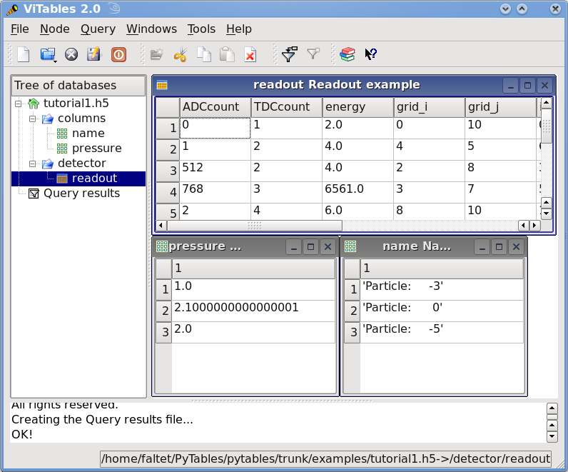
Figure 2. The final version of the data file for tutorial 1.
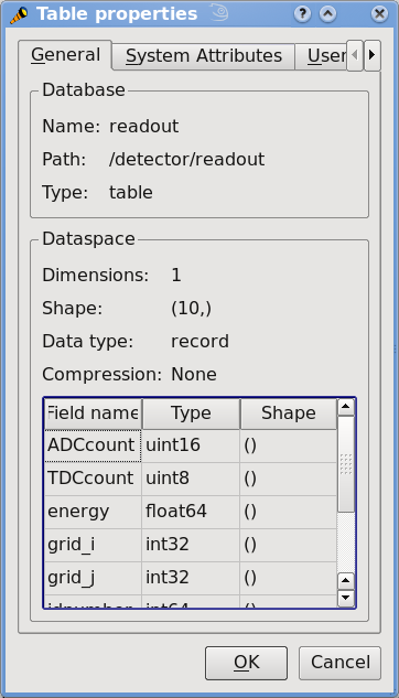
Figure 3. General properties of the /detector/readout table.
Multidimensional table cells and automatic sanity checks
Now it’s time for a more real-life example (i.e. with errors in the code). We will create two groups that branch directly from the root node, Particles and Events. Then, we will put three tables in each group. In Particles we will put tables based on the Particle descriptor and in Events, the tables based the Event descriptor.
Afterwards, we will provision the tables with a number of records. Finally, we will read the newly-created table /Events/TEvent3 and select some values from it, using a comprehension list.
Look at the next script (you can find it in examples/tutorial2.py).
It appears to do all of the above, but it contains some small bugs. Note that
this Particle class is not directly related to the one defined in
last tutorial; this class is simpler (note, however, the multidimensional
columns called pressure and temperature).
We also introduce a new manner to describe a Table as a structured NumPy
dtype (or even as a dictionary), as you can see in the Event description. See
File.create_table() for different kinds of descriptor objects that
can be passed to this method:
import tables as tb
import numpy as np

# Describe a particle record
class Particle(tb.IsDescription):
    name        = tb.StringCol(itemsize=16)  # 16-character string
    lati        = tb.Int32Col()              # integer
    longi       = tb.Int32Col()              # integer
    pressure    = tb.Float32Col(shape=(2,3)) # array of floats (single-precision)
    temperature = tb.Float64Col(shape=(2,3)) # array of doubles (double-precision)

# Native NumPy dtype instances are also accepted
Event = np.dtype([
    ("name"     , "S16"),
    ("TDCcount" , np.uint8),
    ("ADCcount" , np.uint16),
    ("xcoord"   , np.float32),
    ("ycoord"   , np.float32)
    ])

# And dictionaries too (this defines the same structure as above)
# Event = {
#     "name"     : tb.StringCol(itemsize=16),
#     "TDCcount" : tb.UInt8Col(),
#     "ADCcount" : tb.UInt16Col(),
#     "xcoord"   : tb.Float32Col(),
#     "ycoord"   : tb.Float32Col(),
#     }

# Open a file in "w"rite mode
fileh = tb.open_file("tutorial2.h5", mode="w")

# Get the HDF5 root group
root = fileh.root

# Create the groups:
for groupname in ("Particles", "Events"):
    group = fileh.create_group(root, groupname)

# Now, create and fill the tables in Particles group
gparticles = root.Particles

# Create 3 new tables
for tablename in ("TParticle1", "TParticle2", "TParticle3"):
    # Create a table
    table = fileh.create_table("/Particles", tablename, Particle, "Particles: "+tablename)

    # Get the record object associated with the table:
    particle = table.row

    # Fill the table with 257 particles
    for i in range(257):
        # First, assign the values to the Particle record
        particle['name'] = f'Particle: {i:6d}'
        particle['lati'] = i
        particle['longi'] = 10 - i

        ########### Detectable errors start here. Play with them!
        particle['pressure'] = i * np.arange(2 * 4).reshape(2, 4)  # Incorrect
        #particle['pressure'] = i * np.arange(2 * 3).reshape(2, 3) # Correct
        ########### End of errors

        particle['temperature'] = i ** 2     # Broadcasting

        # This injects the Record values
        particle.append()

    # Flush the table buffers
    table.flush()

# Now, go for Events:
for tablename in ("TEvent1", "TEvent2", "TEvent3"):
    # Create a table in Events group
    table = fileh.create_table(root.Events, tablename, Event, "Events: "+tablename)

    # Get the record object associated with the table:
    event = table.row

    # Fill the table with 257 events
    for i in range(257):
        # First, assign the values to the Event record
        event['name']  = f'Event: {i:6d}'
        event['TDCcount'] = i % (1<<8)   # Correct range

        ########### Detectable errors start here. Play with them!
        event['xcoor'] = float(i ** 2)     # Wrong spelling
        #event['xcoord'] = float(i ** 2)   # Correct spelling
        event['ADCcount'] = "sss"        # Wrong type
        #event['ADCcount'] = i * 2       # Correct type
        ########### End of errors

        event['ycoord'] = float(i) ** 4

        # This injects the Record values
        event.append()

    # Flush the buffers
    table.flush()

# Read the records from table "/Events/TEvent3" and select some
table = root.Events.TEvent3
e = [ p['TDCcount'] for p in table if p['ADCcount'] < 20 and 4 <= p['TDCcount'] < 15 ]
print(f"Last record ==> {p}")
print("Selected values ==> {e}")
print("Total selected records ==> {len(e)}")

# Finally, close the file (this also will flush all the remaining buffers!)
fileh.close()
Shape checking
If you look at the code carefully, you’ll see that it won’t work. You will get the following error.
$ python3 tutorial2.py
Traceback (most recent call last):
  File "tutorial2.py", line 60, in <module>
    particle['pressure'] = array(i * arange(2 * 3)).reshape((2, 4))  # Incorrect
ValueError: total size of new array must be unchanged
Closing remaining open files: tutorial2.h5... done
This error indicates that you are trying to assign an array with an incompatible shape to a table cell. Looking at the source, we see that we were trying to assign an array of shape (2,4) to a pressure element, which was defined with the shape (2,3).
In general, these kinds of operations are forbidden, with one valid exception: when you assign a scalar value to a multidimensional column cell, all the cell elements are populated with the value of the scalar. For example:
particle['temperature'] = i ** 2 # Broadcasting
The value i**2 is assigned to all the elements of the temperature table cell. This capability is provided by the NumPy package and is known as broadcasting.
Field name checking
After fixing the previous error and rerunning the program, we encounter another error.
$ python3 tutorial2.py
Traceback (most recent call last):
  File "tutorial2.py", line 73, in ?
    event['xcoor'] = float(i ** 2)     # Wrong spelling
  File "tableextension.pyx", line 1094, in tableextension.Row.__setitem__
  File "tableextension.pyx", line 127, in tableextension.get_nested_field_cache
  File "utilsextension.pyx", line 331, in utilsextension.get_nested_field
KeyError: 'no such column: xcoor'
This error indicates that we are attempting to assign a value to a non-existent field in the event table object. By looking carefully at the Event class attributes, we see that we misspelled the xcoord field (we wrote xcoor instead). This is unusual behavior for Python, as normally when you assign a value to a non-existent instance variable, Python creates a new variable with that name. Such a feature can be dangerous when dealing with an object that contains a fixed list of field names. PyTables checks that the field exists and raises a KeyError if the check fails.
Data type checking
Finally, the last issue which we will find here is a TypeError exception.
$ python3 tutorial2.py
Traceback (most recent call last):
  File "tutorial2.py", line 75, in ?
    event['ADCcount'] = "sss"          # Wrong type
  File "tableextension.pyx", line 1111, in tableextension.Row.__setitem__
TypeError: invalid type (<type 'str'>) for column ``ADCcount``
And, if we change the affected line to read:
event.ADCcount = i * 2 # Correct type
we will see that the script ends well.
You can see the structure created with this (corrected) script in Figure 4. In particular, note the multidimensional column cells in table /Particles/TParticle2.
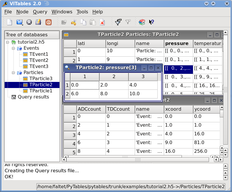
Figure 4. Table hierarchy for tutorial 2.
Using links for more convenient access to nodes
Links are special nodes that can be used to create additional paths to your existing nodes. PyTables supports three kinds of links: hard links, soft links (aka symbolic links) and external links.
Hard links let the user create additional paths to access another node in the same file, and once created, they are indistinguishable from the referred node object, except that they have different paths in the object tree. For example, if the referred node is, say, a Table object, then the new hard link will become a Table object itself. From this point on, you will be able to access the same Table object from two different paths: the original one and the new hard link path. If you delete one path to the table, you will be able to reach it via the other path.
Soft links are similar to hard links, but they keep their own personality. When you create a soft link to another node, you will get a new SoftLink object that refers to that node. However, in order to access the referred node, you need to dereference it.
Finally, external links are like soft links, with the difference that these are meant to point to nodes in external files instead of nodes in the same file. They are represented by the ExternalLink class and, like soft links, you need to dereference them in order to get access to the pointed node.
Interactive example
Now we are going to learn how to deal with links. You can find the code used
in this section in examples/links.py.
First, let’s create a file with some group structure:
>>> import tables as tb
>>> f1 = tb.open_file('links1.h5', 'w')
>>> g1 = f1.create_group('/', 'g1')
>>> g2 = f1.create_group(g1, 'g2')
Now, we will put some datasets on the /g1 and /g1/g2 groups:
>>> a1 = f1.create_carray(g1, 'a1', tb.Int64Atom(), shape=(10000,))
>>> t1 = f1.create_table(g2, 't1', {'f1': tb.IntCol(), 'f2': tb.FloatCol()})
We can start the party now. We are going to create a new group, say /gl, where we will put our links and will start creating one hard link too:
>>> gl = f1.create_group('/', 'gl')
>>> ht = f1.create_hard_link(gl, 'ht', '/g1/g2/t1')  # ht points to t1
>>> print(f"``{ht}`` is a hard link to: ``{t1}``")
``/gl/ht (Table(0,)) `` is a hard link to: ``/g1/g2/t1 (Table(0,)) ``
You can see how we’ve created a hard link in /gl/ht which is pointing to the existing table in /g1/g2/t1. Have look at how the hard link is represented; it looks like a table, and actually, it is a real table. We have two different paths to access that table, the original /g1/g2/t1 and the new one /gl/ht. If we remove the original path we still can reach the table by using the new path:
>>> t1.remove()
>>> print(f"table continues to be accessible in: ``{f1.get_node('/gl/ht')}``")
table continues to be accessible in: ``/gl/ht (Table(0,)) ``
So far so good. Now, let’s create a couple of soft links:
>>> la1 = f1.create_soft_link(gl, 'la1', '/g1/a1')  # la1 points to a1
>>> print(f"``{la1}`` is a soft link to: ``{la1.target}``")
``/gl/la1 (SoftLink) -> /g1/a1`` is a soft link to: ``/g1/a1``
>>> lt = f1.create_soft_link(gl, 'lt', '/g1/g2/t1')  # lt points to t1
>>> print(f"``{lt}`` is a soft link to: ``{lt.target}``")
``/gl/lt (SoftLink) -> /g1/g2/t1 (dangling)`` is a soft link to: ``/g1/g2/t1``
Okay, we see how the first link /gl/la1 points to the array /g1/a1. Notice how the link prints as a SoftLink, and how the referred node is stored in the target instance attribute. The second link (/gt/lt) pointing to /g1/g2/t1 also has been created successfully, but by better inspecting the string representation of it, we see that is labeled as ‘(dangling)’. Why is this? Well, you should remember that we recently removed the /g1/g2/t1 path to access table t1. When printing it, the object knows that it points to nowhere and reports this. This is a nice way to quickly know whether a soft link points to an exiting node or not.
So, let’s re-create the removed path to t1 table:
>>> t1 = f1.create_hard_link('/g1/g2', 't1', '/gl/ht')
>>> print(f"``{lt}`` is not dangling anymore")
``/gl/lt (SoftLink) -> /g1/g2/t1`` is not dangling anymore
and the soft link is pointing to an existing node now.
Of course, for soft links to serve any actual purpose we need a way to get the pointed node. It happens that soft links are callable, and that’s the way to get the referred nodes back:
>>> plt = lt()
>>> print(f"dereferred lt node: ``{plt}``")
dereferred lt node: ``/g1/g2/t1 (Table(0,)) ``
>>> pla1 = la1()
>>> print(f"dereferred la1 node: ``{pla1}``")
dereferred la1 node: ``/g1/a1 (CArray(10000,)) ``
Now, plt is a Python reference to the t1 table while pla1 refers to the a1 array. Easy, uh?
Let’s suppose now that a1 is an array whose access speed is critical for our application. One possible solution is to move the entire file into a faster disk, say, a solid state disk so that access latencies can be reduced quite a lot. However, it happens that our file is too big to fit into our shiny new (although small in capacity) SSD disk. A solution is to copy just the a1 array into a separate file that would fit into our SSD disk. However, our application would be able to handle two files instead of only one, adding significantly more complexity, which is not a good thing.
External links to the rescue! As we’ve already said, external links are like soft links, but they are designed to link objects in external files. Back to our problem, let’s copy the a1 array into a different file:
>>> f2 = tb.open_file('links2.h5', 'w')
>>> new_a1 = a1.copy(f2.root, 'a1')
>>> f2.close()  # close the other file
And now, we can remove the existing soft link and create the external link in its place:
>>> la1.remove()
>>> la1 = f1.create_external_link(gl, 'la1', 'links2.h5:/a1')
>>> print(f"``{la1}`` is an external link to: ``{la1.target}``")
``/gl/la1 (ExternalLink) -> links2.h5:/a1`` is an external link to: ``links2.h5:/a1``
Let’s try dereferring it:
>>> new_a1 = la1()  # dereferrencing la1 returns a1 in links2.h5
>>> print(f"dereferred la1 node:  ``{new_a1}``")
dereferred la1 node:  ``/a1 (CArray(10000,)) ``
Well, it seems like we can access the external node. But just to make sure that the node is in the other file:
>>> print("new_a1 file:", new_a1._v_file.filename)
new_a1 file: links2.h5
Okay, the node is definitely in the external file. So, you won’t have to worry about your application: it will work exactly the same no matter the link is internal (soft) or external.
Finally, here it is a dump of the objects in the final file, just to get a better idea of what we ended with:
>>> f1.close()
>>> exit()
$ ptdump links1.h5
/ (RootGroup) ''
/g1 (Group) ''
/g1/a1 (CArray(10000,)) ''
/gl (Group) ''
/gl/ht (Table(0,)) ''
/gl/la1 (ExternalLink) -> links2.h5:/a1
/gl/lt (SoftLink) -> /g1/g2/t1
/g1/g2 (Group) ''
/g1/g2/t1 (Table(0,)) ''
This ends this tutorial. I hope it helped you to appreciate how useful links can be. I’m sure you will find other ways in which you can use links that better fit your own needs.
Exercising the Undo/Redo feature
PyTables has integrated support for undoing and/or redoing actions. This functionality lets you put marks in specific places of your hierarchy manipulation operations, so that you can make your HDF5 file pop back (undo) to a specific mark (for example for inspecting how your hierarchy looked at that point). You can also go forward to a more recent marker (redo). You can even do jumps to the marker you want using just one instruction as we will see shortly.
You can undo/redo all the operations that are related to object tree management, like creating, deleting, moving or renaming nodes (or complete sub-hierarchies) inside a given object tree. You can also undo/redo operations (i.e. creation, deletion or modification) of persistent node attributes. However, actions which include internal modifications of datasets (that includes Table.append, Table.modify_rows or Table.remove_rows, among others) cannot be currently undone/redone.
This capability can be useful in many situations, for example when doing simulations with multiple branches. When you have to choose a path to follow in such a situation, you can put a mark there and, if the simulation is not going well, you can go back to that mark and start another path. Another possible application is defining coarse-grained operations which operate in a transactional-like way, i.e. which return the database to its previous state if the operation finds some kind of problem while running. You can probably devise many other scenarios where the Undo/Redo feature can be useful to you [3].
A basic example
In this section, we are going to show the basic behavior of the Undo/Redo
feature. You can find the code used in this example in
examples/tutorial3-1.py. A somewhat more complex example will be
explained in the next section.
First, let’s create a file:
>>> import tables
>>> fileh = tables.open_file("tutorial3-1.h5", "w", title="Undo/Redo demo 1")
And now, activate the Undo/Redo feature with the method
File.enable_undo() of File:
>>> fileh.enable_undo()
From now on, all our actions will be logged internally by PyTables. Now, we are going to create a node (in this case an Array object):
>>> one = fileh.create_array('/', 'anarray', [3,4], "An array")
Now, mark this point:
>>> fileh.mark()
1
We have marked the current point in the sequence of actions.
In addition, the mark() method has returned the identifier assigned to this
new mark, that is 1 (mark #0 is reserved for the implicit mark at the
beginning of the action log). In the next section we will see that you can
also assign a name to a mark (see File.mark() for more info on
mark()).
Now, we are going to create another array:
>>> another = fileh.create_array('/', 'anotherarray', [4,5], "Another array")
Right. Now, we can start doing funny things. Let’s say that we want to pop
back to the previous mark (that whose value was 1, do you remember?). Let’s
introduce the undo() method (see File.undo()):
>>> fileh.undo()
Fine, what do you think happened? Well, let’s have a look at the object tree:
>>> print(fileh)
tutorial3-1.h5 (File) 'Undo/Redo demo 1'
Last modif.: 'Tue Mar 13 11:43:55 2007'
Object Tree:
/ (RootGroup) 'Undo/Redo demo 1'
/anarray (Array(2,)) 'An array'
What happened with the /anotherarray node we’ve just created? You’ve guessed it, it has disappeared because it was created after the mark 1. If you are curious enough you may ask - where has it gone? Well, it has not been deleted completely; it has just been moved into a special, hidden group of PyTables that renders it invisible and waiting for a chance to be reborn.
Now, unwind once more, and look at the object tree:
>>> fileh.undo()
>>> print(fileh)
tutorial3-1.h5 (File) 'Undo/Redo demo 1'
Last modif.: 'Tue Mar 13 11:43:55 2007'
Object Tree:
/ (RootGroup) 'Undo/Redo demo 1'
Oops, /anarray has disappeared as well!
Don’t worry, it will visit us again very shortly. So, you might be somewhat lost
right now; at which mark are we? Let’s ask the File.get_current_mark()
method in the file handler:
>>> print(fileh.get_current_mark())
0
So we are at mark #0, remember? Mark #0 is an implicit mark that is created
when you start the log of actions when calling File.enable_undo(). Fine, but
you are missing your too-young-to-die arrays. What can we do about that?
File.redo() to the rescue:
>>> fileh.redo()
>>> print(fileh)
tutorial3-1.h5 (File) 'Undo/Redo demo 1'
Last modif.: 'Tue Mar 13 11:43:55 2007'
Object Tree:
/ (RootGroup) 'Undo/Redo demo 1'
/anarray (Array(2,)) 'An array'
Great! The /anarray array has come into life again. Just check that it is alive and well:
>>> fileh.root.anarray.read()
[3, 4]
>>> fileh.root.anarray.title
'An array'
Well, it looks pretty similar to its past life; what’s more, it is exactly the same object:
>>> fileh.root.anarray is one
True
It was just moved to the hidden group and back again, that’s all! That’s kind of fun, so we are going to do the same with /anotherarray:
>>> fileh.redo()
>>> print(fileh)
tutorial3-1.h5 (File) 'Undo/Redo demo 1'
Last modif.: 'Tue Mar 13 11:43:55 2007'
Object Tree:
/ (RootGroup) 'Undo/Redo demo 1'
/anarray (Array(2,)) 'An array'
/anotherarray (Array(2,)) 'Another array'
Welcome back, /anotherarray! Just a couple of sanity checks:
>>> assert fileh.root.anotherarray.read() == [4,5]
>>> assert fileh.root.anotherarray.title == "Another array"
>>> fileh.root.anotherarray is another
True
Nice, you managed to turn your data back to life. Congratulations! But wait, do not forget to close your action log when you don’t need this feature anymore:
>>> fileh.disable_undo()
That will allow you to continue working with your data without actually requiring PyTables to keep track of all your actions, and more importantly, allowing your objects to die completely if they have to, not requiring to keep them anywhere, hence saving process time and space in your database file.
A more complete example
Now, time for a somewhat more sophisticated demonstration of the Undo/Redo
feature. In it, several marks will be set in different parts of the code flow
and we will see how to jump between these marks with just one method call.
You can find the code used in this example in examples/tutorial3-2.py
Let’s introduce the first part of the code:
import tables

# Create an HDF5 file
fileh = tables.open_file('tutorial3-2.h5', 'w', title='Undo/Redo demo 2')

        #'-**-**-**-**-**-**- enable undo/redo log  -**-**-**-**-**-**-**-'
fileh.enable_undo()

# Start undoable operations
fileh.create_array('/', 'otherarray1', [3,4], 'Another array 1')
fileh.create_group('/', 'agroup', 'Group 1')

# Create a 'first' mark
fileh.mark('first')
fileh.create_array('/agroup', 'otherarray2', [4,5], 'Another array 2')
fileh.create_group('/agroup', 'agroup2', 'Group 2')

# Create a 'second' mark
fileh.mark('second')
fileh.create_array('/agroup/agroup2', 'otherarray3', [5,6], 'Another array 3')

# Create a 'third' mark
fileh.mark('third')
fileh.create_array('/', 'otherarray4', [6,7], 'Another array 4')
fileh.create_array('/agroup', 'otherarray5', [7,8], 'Another array 5')
You can see how we have set several marks interspersed in the code flow, representing different states of the database. Also, note that we have assigned names to these marks, namely ‘first’, ‘second’ and ‘third’.
Now, start doing some jumps back and forth in the states of the database:
# Now go to mark 'first'
fileh.goto('first')
assert '/otherarray1' in fileh
assert '/agroup' in fileh
assert '/agroup/agroup2' not in fileh
assert '/agroup/otherarray2' not in fileh
assert '/agroup/agroup2/otherarray3' not in fileh
assert '/otherarray4' not in fileh
assert '/agroup/otherarray5' not in fileh

# Go to mark 'third'
fileh.goto('third')
assert '/otherarray1' in fileh
assert '/agroup' in fileh
assert '/agroup/agroup2' in fileh
assert '/agroup/otherarray2' in fileh
assert '/agroup/agroup2/otherarray3' in fileh
assert '/otherarray4' not in fileh
assert '/agroup/otherarray5' not in fileh

# Now go to mark 'second'
fileh.goto('second')
assert '/otherarray1' in fileh
assert '/agroup' in fileh
assert '/agroup/agroup2' in fileh
assert '/agroup/otherarray2' in fileh
assert '/agroup/agroup2/otherarray3' not in fileh
assert '/otherarray4' not in fileh
assert '/agroup/otherarray5' not in fileh
Well, the code above shows how easy is to jump to a certain mark in the
database by using the File.goto() method.
There are also a couple of implicit marks for going to the beginning or the end of the saved states: 0 and -1. Going to mark #0 means go to the beginning of the saved actions, that is, when method fileh.enable_undo() was called. Going to mark #-1 means go to the last recorded action, that is the last action in the code flow.
Let’s see what happens when going to the end of the action log:
# Go to the end
fileh.goto(-1)
assert '/otherarray1' in fileh
assert '/agroup' in fileh
assert '/agroup/agroup2' in fileh
assert '/agroup/otherarray2' in fileh
assert '/agroup/agroup2/otherarray3' in fileh
assert '/otherarray4' in fileh
assert '/agroup/otherarray5' in fileh

# Check that objects have come back to life in a sane state
assert fileh.root.otherarray1.read() == [3,4]
assert fileh.root.agroup.otherarray2.read() == [4,5]
assert fileh.root.agroup.agroup2.otherarray3.read() == [5,6]
assert fileh.root.otherarray4.read() == [6,7]
assert fileh.root.agroup.otherarray5.read() == [7,8]
Try going to the beginning of the action log yourself (remember, mark #0) and check contents of the object tree.
We have nearly finished this demonstration. As always, do not forget to close the action log as well as the database:
#'-**-**-**-**-**-**- disable undo/redo log  -**-**-**-**-**-**-**-'
fileh.disable_undo()
# Close the file
fileh.close()
You might want to check other examples on Undo/Redo feature that appear in
examples/undo-redo.py.
Using enumerated types
PyTables includes support for handling enumerated types. Those types are defined by providing an exhaustive set or list of possible, named values for a variable of that type. Enumerated variables of the same type are usually compared between them for equality and sometimes for order, but are not usually operated upon.
Enumerated values have an associated name and concrete value. Every name is unique and so are concrete values. An enumerated variable always takes the concrete value, not its name. Usually, the concrete value is not used directly, and frequently it is entirely irrelevant. For the same reason, an enumerated variable is not usually compared with concrete values out of its enumerated type. For that kind of use, standard variables and constants are more adequate.
PyTables provides the Enum (see The Enum class) class to provide support for enumerated types. Each instance of Enum is an enumerated type (or enumeration). For example, let us create an enumeration of colors
All these examples can be found in examples/play-with-enums.py:
>>> import tables
>>> colorList = ['red', 'green', 'blue', 'white', 'black']
>>> colors = tables.Enum(colorList)
Here we used a simple list giving the names of enumerated values, but we left the choice of concrete values up to the Enum class. Let us see the enumerated pairs to check those values:
>>> print("Colors:", [v for v in colors])
Colors: [('blue', 2), ('black', 4), ('white', 3), ('green', 1), ('red', 0)]
Names have been given automatic integer concrete values. We can iterate over values in an enumeration, but we will usually be more interested in accessing single values. We can get the concrete value associated with a name by accessing it as an attribute or as an item (the later can be useful for names not resembling Python identifiers):
>>> print("Value of 'red' and 'white':", (colors.red, colors.white))
Value of 'red' and 'white': (0, 3)
>>> print("Value of 'yellow':", colors.yellow)
Value of 'yellow':
Traceback (most recent call last):
  File "<stdin>", line 1, in ?
  File ".../tables/misc/enum.py", line 230, in __getattr__
    raise AttributeError(\*ke.args)
AttributeError: no enumerated value with that name: 'yellow'
>>>
>>> print("Value of 'red' and 'white':", (colors['red'], colors['white']))
Value of 'red' and 'white': (0, 3)
>>> print("Value of 'yellow':", colors['yellow'])
Value of 'yellow':
Traceback (most recent call last):
  File "<stdin>", line 1, in ?
  File ".../tables/misc/enum.py", line 189, in __getitem__
    raise KeyError("no enumerated value with that name: %r" % (name,))
KeyError: "no enumerated value with that name: 'yellow'"
See how accessing a value that is not in the enumeration raises the appropriate exception. We can also do the opposite and get the name that matches a concrete value by using the __call__() method of Enum:
>>> print(f"Name of value {colors.red}:", colors(colors.red))
Name of value 0: red
>>> print("Name of value 1234:", colors(1234))
Name of value 1234:
Traceback (most recent call last):
  File "<stdin>", line 1, in ?
  File ".../tables/misc/enum.py", line 320, in __call__
    raise ValueError(
ValueError: no enumerated value with that concrete value: 1234
You can see what we made as using the enumerated type to convert a concrete value into a name in the enumeration. Of course, values out of the enumeration can not be converted.
Enumerated columns
Columns of an enumerated type can be declared by using the EnumCol (see The Col class and its descendants) class. To see how this works, let us open a new PyTables file and create a table to collect the simulated results of a probabilistic experiment. In it, we have a bag full of colored balls; we take a ball out and annotate the time of extraction and the color of the ball:
>>> h5f = tables.open_file('enum.h5', 'w')
>>> class BallExt(tables.IsDescription):
...     ballTime = tables.Time32Col()
...     ballColor = tables.EnumCol(colors, 'black', base='uint8')
>>> tbl = h5f.create_table('/', 'extractions', BallExt, title="Random ball extractions")
>>>
We declared the ballColor column to be of the enumerated type colors, with a default value of black. We also stated that we are going to store concrete values as unsigned 8-bit integer values [4].
Let us use some random values to fill the table:
>>> import time
>>> import random
>>> now = time.time()
>>> row = tbl.row
>>> for i in range(10):
...     row['ballTime'] = now + i
...     row['ballColor'] = colors[random.choice(colorList)]  # take note of this
...     row.append()
>>>
Notice how we used the __getitem__() call of colors to get the concrete value to store in ballColor. This way of appending values to a table automatically checks for the validity on enumerated values. For instance:
>>> row['ballTime'] = now + 42
>>> row['ballColor'] = 1234
Traceback (most recent call last):
  File "<stdin>", line 1, in <module>
  File "tableextension.pyx", line 1086, in tableextension.Row.__setitem__
  File ".../tables/misc/enum.py", line 320, in __call__
    "no enumerated value with that concrete value: %r" % (value,))
ValueError: no enumerated value with that concrete value: 1234
Note that this check is performed only by row.append() and not in other methods such as tbl.append() or tbl.modify_rows(). Now, after flushing the table we can see the result of insertions:
>>> tbl.flush()
>>> for r in tbl:
...     ballTime = r['ballTime']
...     ballColor = colors(r['ballColor'])  # notice this
...     print("Ball extracted on %d is of color %s." % (ballTime, ballColor))
Ball extracted on 1173785568 is of color green.
Ball extracted on 1173785569 is of color black.
Ball extracted on 1173785570 is of color white.
Ball extracted on 1173785571 is of color black.
Ball extracted on 1173785572 is of color black.
Ball extracted on 1173785573 is of color red.
Ball extracted on 1173785574 is of color green.
Ball extracted on 1173785575 is of color red.
Ball extracted on 1173785576 is of color white.
Ball extracted on 1173785577 is of color white.
As a final note, you may be wondering how to access an enumeration associated
with ballColor once the file is closed and reopened. You can call tbl.get_enum(‘ballColor’)
(see Table.get_enum()) to get the enumeration back.
Enumerated arrays
EArray and VLArray leaves can also be declared to store enumerated values by means of the EnumAtom (see The Atom class and its descendants) class, which works very much like EnumCol for tables. Also, Array leaves can be used to open native HDF enumerated arrays.
Let us create a sample EArray containing ranges of working days as bidimensional values:
>>> workingDays = {'Mon': 1, 'Tue': 2, 'Wed': 3, 'Thu': 4, 'Fri': 5}
>>> dayRange = tables.EnumAtom(workingDays, 'Mon', base='uint16')
>>> earr = h5f.create_earray('/', 'days', dayRange, (0, 2), title="Working day ranges")
>>> earr.flavor = 'python'
Nothing unusual, except for two details. Firstly, we use a dictionary instead of a list to explicitly set concrete values in the enumeration. Secondly, there is no explicit Enum instance created! Instead, the dictionary is passed as the first argument to the constructor of EnumAtom. If the constructor receives a list or a dictionary instead of an enumeration, it automatically builds the enumeration from it.
Now let us feed some data to the array:
>>> wdays = earr.get_enum()
>>> earr.append([(wdays.Mon, wdays.Fri), (wdays.Wed, wdays.Fri)])
>>> earr.append([(wdays.Mon, 1234)])
Please note that, since we had no explicit Enum instance, we were forced to use get_enum() (see EArray methods) to get it from the array (we could also have used dayRange.enum). Also note that we were able to append an invalid value (1234). Array methods do not check the validity of enumerated values.
Finally, we will print contents of the array:
>>> for (d1, d2) in earr:
...     print(f"From {wdays(d1) to {wdays(d2) ({d2 - d1 + 1} days).")
From Mon to Fri (5 days).
From Wed to Fri (3 days).
Traceback (most recent call last):
  File "<stdin>", line 2, in <module>
  File ".../tables/misc/enum.py", line 320, in __call__
    "no enumerated value with that concrete value: %r" % (value,))
ValueError: no enumerated value with that concrete value: 1234
That was an example of operating on concrete values. It also showed how the value-to-name conversion failed because of the value not belonging to the enumeration.
Now we will close the file, and this little tutorial on enumerated types is done:
>>> h5f.close()
Nested structures in tables
PyTables supports handling of nested structures (or, in other words, nested datatypes) in table objects, allowing you to define nested columns of arbitrary depth.
Why is that useful? Suppose your data has a certain structure on the column level, which you would like to represent in the data model. You can do so by creating nested subclasses of IsDescription. The benefit is the ability to group and retrieve data more easily. Example below may be a bit silly, but it will serve as an illustration of the concept:
import tables as tb

class Info(tb.IsDescription):
    """A sub-structure of NestedDescr"""
    _v_pos = 2   # The position in the whole structure
    name = tb.StringCol(10)
    value = tb.Float64Col(pos=0)

colors = tb.Enum(['red', 'green', 'blue'])

class NestedDescr(tb.IsDescription):
    """A description that has several nested columns"""
    color = tb.EnumCol(colors, 'red', base='uint32')
    info1 = tb.Info()

    class info2(tb.IsDescription):
        _v_pos = 1
        name = tb.StringCol(10)
        value = tb.Float64Col(pos=0)

        class info3(tb.IsDescription):
            x = tb.Float64Col(dflt=1)
            y = tb.UInt8Col(dflt=1)
NestedDescr is the root class with two substructures in it: info1 and info2. Note info1 is an instance of class Info which is defined prior to NestedDescr. info2 is declared within NestedDescr. Also, there is a third substructure, info3, that is in turn declared within substructure info2. You can define positions of substructures in the containing object by declaring special class attribute _v_pos.
Creating nested tables
Now that we have defined our nested structure, let’s create a nested table, that is a table with columns which contain subcolumns:
>>> fileh = tb.open_file("nested-tut.h5", "w")
>>> table = fileh.create_table(fileh.root, 'table', NestedDescr)
Done! Now, to populate the table with values, assign a value to each field. Referencing nested fields can be accomplished by providing a full path. Follow the structure defined earlier - use ‘/’ to access each sublevel of the structure, similar to how you would access a subdirectory on a Unix filesystem:
>>> row = table.row
>>> for i in range(10):
...     row['color'] = colors[['red', 'green', 'blue'][i % 3]]
...     row['info1/name'] = f"name1-{i}"
...     row['info2/name'] = f"name2-{i}"
...     row['info2/info3/y'] =  i
...     # Remaining fields will be filled with defaults
...     row.append()
>>> table.flush()
>>> table.nrows
10
As demonstrated above, substructure’s field can be accessed by specifying its full path as defined in the table hierarchy.
Reading nested tables
Now, what happens if we want to read the table? What kind of data container would we get? Let’s find out:
>>> nra = table[::4]
>>> nra
array([(((1.0, 0), 'name2-0', 0.0), ('name1-0', 0.0), 0L),
       (((1.0, 4), 'name2-4', 0.0), ('name1-4', 0.0), 1L),
       (((1.0, 8), 'name2-8', 0.0), ('name1-8', 0.0), 2L)],
       dtype=[('info2', [('info3', [('x', '>f8'), ('y', '\|u1')]),
              ('name', '\|S10'), ('value', '>f8')]),
              ('info1', [('name', '\|S10'), ('value', '>f8')]),
              ('color', '>u4')])
What we’ve got is a NumPy array with a compound, nested datatype, i.e. its dtype is a list of name-datatype tuples. For every fourth row in the table (note [::4]), we get one resulting row, giving a total of three.
You can make use of the above object in many different ways. For example, you can use it to append new data to an existing table object:
>>> table.append(nra)
>>> table.nrows
13
Or to create new tables:
>>> table2 = fileh.create_table(fileh.root, 'table2', nra)
>>> table2[:]
array([(((1.0, 0), 'name2-0', 0.0), ('name1-0', 0.0), 0L),
       (((1.0, 4), 'name2-4', 0.0), ('name1-4', 0.0), 1L),
       (((1.0, 8), 'name2-8', 0.0), ('name1-8', 0.0), 2L)],
       dtype=[('info2', [('info3', [('x', '<f8'), ('y', '\|u1')]),
              ('name', '\|S10'), ('value', '<f8')]),
              ('info1', [('name', '\|S10'), ('value', '<f8')]),
              ('color', '<u4')])
Finally, you can select nested values that meet an arbitrary condition:
>>> names = [ x['info2/name'] for x in table if x['color'] == colors.red ]
>>> names
['name2-0', 'name2-3', 'name2-6', 'name2-9', 'name2-0']
Note that row accessor does not provide natural naming feature, so you have to specify an absolute path to your desired column in order to access it.
Using Cols accessor
We can use cols attribute object (see The Cols class) of the table to conveniently access data stored in a substructure:
>>> table.cols.info2[1:5]
array([((1.0, 1), 'name2-1', 0.0), ((1.0, 2), 'name2-2', 0.0),
       ((1.0, 3), 'name2-3', 0.0), ((1.0, 4), 'name2-4', 0.0)],
       dtype=[('info3', [('x', '<f8'), ('y', '\|u1')]), ('name', '\|S10'),
              ('value', '<f8')])
Here, we have made use of the cols accessor to access info2 substructure and a slice operation to retrieve a subset of data we were interested in; you probably recognized natural naming approach used here as well. We can continue and ask for data in info3 substructure:
>>> table.cols.info2.info3[1:5]
array([(1.0, 1), (1.0, 2), (1.0, 3), (1.0, 4)],
       dtype=[('x', '<f8'), ('y', '\|u1')])
You can also use the _f_col method to get a handler for the column:
>>> table.cols._f_col('info2')
/table.cols.info2 (Cols), 3 columns
  info3 (Cols(), Description)
  name (Column(), \|S10)
  value (Column(), float64)
Here, you’ve got another Cols object handler because info2 was a nested column. If you select a non-nested column, you will get a regular Column instance:
>>> table.cols._f_col('info2/info3/y')
/table.cols.info2.info3.y (Column(), uint8, idx=None)
To summarize, cols accessor is a very handy and powerful tool to access data in nested tables. Don’t hesitate to use it, especially when doing interactive work.
Accessing meta-information of nested tables
Tables have a description attribute, which returns an instance of the Description class (see The Description class) with table meta-data. It can be helpful in understanding the table structure, including nested columns:
>>> table.description
{
  "info2": {
    "info3": {
      "x": Float64Col(shape=(), dflt=1.0, pos=0),
      "y": UInt8Col(shape=(), dflt=1, pos=1)},
    "name": StringCol(itemsize=10, shape=(), dflt='', pos=1),
    "value": Float64Col(shape=(), dflt=0.0, pos=2)},
  "info1": {
    "name": StringCol(itemsize=10, shape=(), dflt='', pos=0),
    "value": Float64Col(shape=(), dflt=0.0, pos=1)},
  "color": EnumCol(enum=Enum({'blue': 2, 'green': 1, 'red': 0}), dflt='red',
                   base=UInt32Atom(shape=(), dflt=0), shape=(), pos=2)}
As you can see, it provides very useful information on both the format and the structure of columns in your table.
You can use natural naming approach with the description attribute to gain access to subcolumn’s meta-data:
>>> table.description.info1
{"name": StringCol(itemsize=10, shape=(), dflt='', pos=0),
 "value": Float64Col(shape=(), dflt=0.0, pos=1)}
>>> table.description.info2.info3
{"x": Float64Col(shape=(), dflt=1.0, pos=0),
 "y": UInt8Col(shape=(), dflt=1, pos=1)}
_v_nested_names attribute provides names of columns as well as structures embedded in them:
>>> table.description._v_nested_names
[('info2', [('info3', ['x', 'y']), 'name', 'value']),
 ('info1', ['name', 'value']), 'color']
>>> table.description.info1._v_nested_names
['name', 'value']
Regardless of which level of the structure is accessed, the output of _v_nested_names contains the same kind of information. This is because even for nested structures, a Description object is returned.
It is possible to create arrays that immitate nested table-like structure with _v_nested_descr attribute:
>>> import numpy as np
>>> table.description._v_nested_descr
[('info2', [('info3', [('x', '()f8'), ('y', '()u1')]), ('name', '()S10'),
 ('value', '()f8')]), ('info1', [('name', '()S10'), ('value', '()f8')]),
 ('color', '()u4')]
>>> np.rec.array(None, shape=0, dtype=table.description._v_nested_descr)
recarray([],
      dtype=[('info2', [('info3', [('x', '>f8'), ('y', '|u1')]),
             ('name', '|S10'), ('value', '>f8')]),
             ('info1', [('name', '|S10'), ('value', '>f8')]),
             ('color', '>u4')])
>>> np.rec.array(
        None, shape=0, dtype=table.description.info2._v_nested_descr
    )
recarray([],
      dtype=[('info3', [('x', '>f8'), ('y', '|u1')]), ('name', '|S10'),
             ('value', '>f8')])
Last but not least, there is a special iterator of the Description class: _f_walk, which returns different columns of the table:
>>> for coldescr in table.description._f_walk():
...     print(f"column--> {coldescr}")
column--> Description([('info2', [('info3', [('x', '()f8'), ('y', '()u1')]),
                       ('name', '()S10'), ('value', '()f8')]),
                       ('info1', [('name', '()S10'), ('value', '()f8')]),
                       ('color', '()u4')])
column--> EnumCol(enum=Enum({'blue': 2, 'green': 1, 'red': 0}), dflt='red',
                            base=UInt32Atom(shape=(), dflt=0), shape=(), pos=2)
column--> Description([('info3', [('x', '()f8'), ('y', '()u1')]), ('name', '()S10'),
                       ('value', '()f8')])
column--> StringCol(itemsize=10, shape=(), dflt='', pos=1)
column--> Float64Col(shape=(), dflt=0.0, pos=2)
column--> Description([('name', '()S10'), ('value', '()f8')])
column--> StringCol(itemsize=10, shape=(), dflt='', pos=0)
column--> Float64Col(shape=(), dflt=0.0, pos=1)
column--> Description([('x', '()f8'), ('y', '()u1')])
column--> Float64Col(shape=(), dflt=1.0, pos=0)
column--> UInt8Col(shape=(), dflt=1, pos=1)
See the The Description class for a complete listing of attributes and methods of the Description object.
Well, this is the end of this tutorial. As always, remember to close your files:
>>> fileh.close()
Finally, you may want to have a look at your resulting data file.
$ ptdump -d nested-tut.h5
/ (RootGroup) ''
/table (Table(13,)) ''
  Data dump:
[0] (((1.0, 0), 'name2-0', 0.0), ('name1-0', 0.0), 0L)
[1] (((1.0, 1), 'name2-1', 0.0), ('name1-1', 0.0), 1L)
[2] (((1.0, 2), 'name2-2', 0.0), ('name1-2', 0.0), 2L)
[3] (((1.0, 3), 'name2-3', 0.0), ('name1-3', 0.0), 0L)
[4] (((1.0, 4), 'name2-4', 0.0), ('name1-4', 0.0), 1L)
[5] (((1.0, 5), 'name2-5', 0.0), ('name1-5', 0.0), 2L)
[6] (((1.0, 6), 'name2-6', 0.0), ('name1-6', 0.0), 0L)
[7] (((1.0, 7), 'name2-7', 0.0), ('name1-7', 0.0), 1L)
[8] (((1.0, 8), 'name2-8', 0.0), ('name1-8', 0.0), 2L)
[9] (((1.0, 9), 'name2-9', 0.0), ('name1-9', 0.0), 0L)
[10] (((1.0, 0), 'name2-0', 0.0), ('name1-0', 0.0), 0L)
[11] (((1.0, 4), 'name2-4', 0.0), ('name1-4', 0.0), 1L)
[12] (((1.0, 8), 'name2-8', 0.0), ('name1-8', 0.0), 2L)
/table2 (Table(3,)) ''
  Data dump:
[0] (((1.0, 0), 'name2-0', 0.0), ('name1-0', 0.0), 0L)
[1] (((1.0, 4), 'name2-4', 0.0), ('name1-4', 0.0), 1L)
[2] (((1.0, 8), 'name2-8', 0.0), ('name1-8', 0.0), 2L)
Most of the code in this section is also available in
examples/nested-tut.py.
PyTables provides a comprehensive set of tools to work with nested structures and to address your classification needs. Try to avoid nesting your data too deeply as it may lead to very long and convoluted series of lists, tuples, and description objects, which can be hard to read and understand.
Other examples in PyTables distribution
Feel free to examine the rest of examples in directory examples/, and
try to understand them. We have written several practical sample scripts to
give you an idea of the PyTables capabilities, its way of dealing with HDF5
objects, and how it can be used in the real world.